Chapter 5 Node Calibration
In the previous chapter we saw that various ways that the node gps can differ, which can lead to inaccurate received signal strength indicators (RSSI) from the tag.
To account for any small changes in the gps values, we need to calibrate the node grid. ## Load library
5.1 Load sidekick data file
Place the .csv file generated by the CTT Sidekick into the sidekick folder:
# Specify the path to the sidekick data file you recorded for calibration
# it is best if you create a 'sidekick' folder to store your calibration file(s).

create_outpath('./data/Meadows V2/sidekick/')
The celltracktech package comes with the sidekick calibration file from the Meadows V2 site. For the purposes of this tutorial, we will save it as a .csv file and place it in the sidekick folder. If you were using your data, you would need to place the sidekick calibration file manuall in the sidekick folder.
write_csv(celltracktech::sidekick_cal, './data/Meadows V2/sidekick/calibration.csv')

sidekick_file_path <- './data/Meadows V2/sidekick/calibration.csv'
5.1.1 IF YOU DO NOT HAVE A SIDEKICK DATA FILE:
Create your own sidekick file by walking with a tag through node grid, stopping at specific spots you choose, and note the gps coordinates and time. Then create a csv similar to the sidekick calibration file.
Example:
| tag_type | tag_id | time_utc | rssi | lat | lon | heading | antenna_angle |
|---|---|---|---|---|---|---|---|
| radio434mhz | 4C34074B | 2023-08-03 19:42:44.721001Z | 38.935561 | -74.948195 | 24.273 | ||
| radio434mhz | 072A6633 | 2023-08-03 19:42:45.307456Z | 38.935561 | -74.948195 | 23.548 | ||
| radio434mhz | 19332A07 | 2023-08-03 19:42:48.366123Z | 38.935569 | -74.948195 | 15.840 |
5.2 Setup
5.2.2 Load settings
# Settings - ----------------------------------------------------------------

# set significant digits (number of digits after decimal)
options(digits = 10)

# These were created in Chapter 2. If you do not have these in your project directory, go back and repeat Ch. 2.
my_token <- Sys.getenv('API_KEY') # load env variable into my_token
myproject <- "Meadows V2" # this is your project name on your CTT account, here we are using the CTT project 'Meadows V2'
outpath <- "./data/" # where your downloaded files are to go

# Specify the path to your database file
database_file <- "./data/Meadows V2/meadows.duckdb"

# Specify the tag ID that you used in your calibration
my_tag_id <- "072A6633"
# my_tag_id <- "614B661E"

# Specify the time range of node data you want to import for this analysis
#   This range should cover a large time window where you nodes were in
#   a constant location.  All node health records in this time window
#   will be used to accurately determine the position of your nodes
start_time <- as.POSIXct("2023-08-01 00:00:00", tz = "GMT")
stop_time <- as.POSIXct("2023-08-07 00:00:00", tz = "GMT")

# Specify a list of node Ids if you only want to include a subset in calibration
# IF you want to use all nodes, ignore this line and SKIP the step below
# where the data frame is trimmed to only nodes in this list
my_nodes <- c("B25AC19E", "44F8E426", "FAB6E12", "1EE02113", "565AA5B9", "EE799439", "1E762CF3", "A837A3F4", "484ED33B")

# You can specify an alternative map tile URL to use here
my_tile_url <- "https://mt2.google.com/vt/lyrs=y&x={x}&y={y}&z={z}"
5.2.3 Load Node Health Data from Files
# connect to the database
con <- DBI::dbConnect(duckdb::duckdb(),
                      dbdir = database_file,
                      read_only = TRUE)

# load node_health table in to RStudio and subset it based on your start and stop times
node_health_df <- tbl(con, "node_health") |>
  filter(time >= start_time & time <= stop_time) |>
  collect()

# disconnect from the database
DBI::dbDisconnect(con)

# remove any duplicate records
node_health_df <- node_health_df %>%
  distinct(node_id,
           time,
           recorded_at,
           .keep_all = TRUE)
5.2.4 Get Node Locations
# Calculate the average node locations
node_locs <- calculate_node_locations(node_health_df)

# Plot the average node locations
node_loc_plot <- plot_node_locations(node_health_df,
                                     node_locs,
                                     theme = classic_plot_theme())
node_loc_plot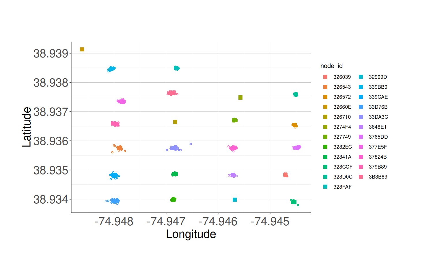
# Write the node locations to a file
create_outpath('results')

export_node_locations("results/node_locations.csv",
                      node_locs)

# Draw a map with the node locations
node_map <- map_node_locations(node_locs,
                               tile_url = my_tile_url)
node_map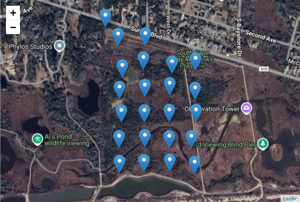
5.2.5 Load Station Detection from Files
# connect to database
con <- DBI::dbConnect(duckdb::duckdb(),
                      dbdir = database_file,
                      read_only = TRUE)

# load raw data table and filter from start_time to stop_time
detection_df <- tbl(con, "raw") |>
  filter(time >= start_time && time <= stop_time) |>
  collect()

# if you are working with blu data, uncomment the lines below and load data from the blu table
# detection_blu <- tbl(con, "blu") |>
#   filter(time >= start_time && time <= stop_time) |>
#   collect

# disconnect from database
DBI::dbDisconnect(con)

# Get beeps from test tag only
detection_df <- subset.data.frame(detection_df,
                                  tag_id == my_tag_id)
5.2.6 Load Sidekick Calibration Data
# Get Sidekick data from CSV
sidekick_all_df <- load_sidekick_data(sidekick_file_path)

# Get beeps from test tag only
sidekick_tag_df <- subset.data.frame(sidekick_all_df,
                                     tag_id == my_tag_id)

# Show location of all beeps in relation to node locations
calibration_map <- map_calibration_track(node_locs,
                                         sidekick_tag_df,
                                         tile_url = my_tile_url)

calibration_map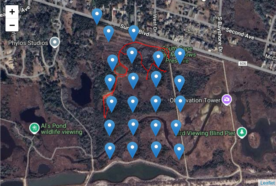
5.3 Calculate the RSSI vs. Distance Relationship
This function will match sidekick detections to detections recorded by nodes and sent to the station. Then using the sidekick location, the node locations calculated above, and the rssi measured in the node, a list of rssi and distance pairs is generated and returned.
For Blu Series tags use_sync=TRUE, for 434 MHz tags use_sync=FALSE.
rssi_v_dist <- calc_rssi_v_dist(node_locs = node_locs,
                                sidekick_tag_df = sidekick_tag_df,
                                detection_df = detection_df,
                                use_sync = FALSE)

# Plot the resulting RSSI and distance data
ggplot() +
  geom_point(data = rssi_v_dist,
             aes(x = distance,
                 y = rssi,
                 colour = node_id)) +
  labs(title="RSSI vs. Distance",
       x="Distance (m)",
       y="RSSI (dBm)",
       colour="Node ID") +
  classic_plot_theme()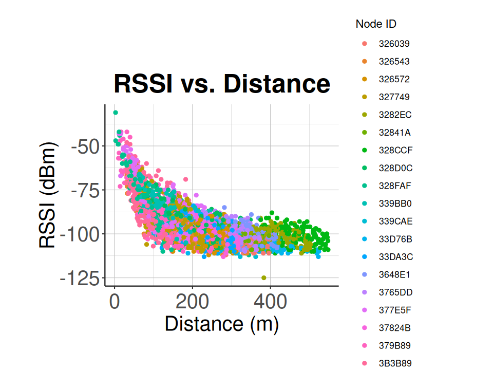
# Fit the RSSI vs distance data with exponential relationship
nlsfit <- nls(
  rssi ~ a - b * exp(-c * distance),
  rssi_v_dist,
  start = list(a = -105, b = -60, c = 0.17)
)

summary(nlsfit)

# Get the coefficients from the fit result
co <- coef(summary(nlsfit))
rssi_coefs <- c(co[1, 1], co[2, 1], co[3, 1])

# Add a predicted column to the RSSI vs distance data
rssi_v_dist$pred <- predict(nlsfit)

# Plot the RSSI vs distance data with the fit curve
calibration_plot <- plot_calibration_result(rssi_v_dist, classic_plot_theme())
calibration_plot

# Print the coefficients from the fit. You'll need these coefficients later
# for localization.
print(rssi_coefs)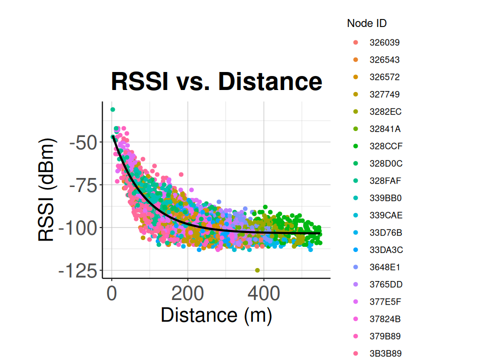
Your node grid is now calibrated!