Chapter 8 Habitat Use
Calculate where an animal spends its time.
8.1 Load libraries and settings
8.1.4 Load RSSI Coefficients
Remember Chapter 5 in which we calibrated the node grid? We will want to use those RSSI coefficients to accurately calculate the tag tracks from the detection data.
We will set the coefficients in the code block below, as well as our start and stop time for the Nodes, and for the tag detections.
8.1.5 Load Settings
options(digits = 10)

# Specify the time range of node data you want to import for this analysis
#   This range should cover a large time window where your nodes were in
#   a constant location.  All node health records in this time window
#   will be used to accurately determine the position of your nodes
node_start_time <- as.POSIXct("2023-08-01 00:00:00", tz = "GMT")
node_stop_time <- as.POSIXct("2023-08-07 00:00:00", tz = "GMT")

# Selected Tag Id - Hybrid tag on a Gray Catbird (GRCA)
selected_tag_id <- '2A33611E' # tag with most detections, 1/4 wave

# Analysis Time Range
det_start_time <- as.POSIXct("2023-10-01 12:00:00", tz = "GMT")
det_stop_time <- as.POSIXct("2023-10-06 12:00:00", tz = "GMT")

# You can specify an alternative map tile URL to use here
my_tile_url <- "https://mt2.google.com/vt/lyrs=y&x={x}&y={y}&z={z}"
8.2 Load Node Health Data from Files
# Load from DB
con <- DBI::dbConnect(duckdb::duckdb(),
                      dbdir = database_file,
                      read_only = TRUE)

# load node_health data table into RStudio and filter it based on the start and stop time
node_health_df <- tbl(con, "node_health") |>
  filter(time >= node_start_time && time <= node_stop_time) |>
  collect()

# disconnect from the database
DBI::dbDisconnect(con)

# Remove duplicates
node_health_df <- node_health_df %>%
  distinct(node_id,
           time,
           recorded_at,
           .keep_all = TRUE)
8.3 Get Node Locations
Due to variations in GPS coordinates, it is a good idea to plot the Node locations and overlay the plot over a satellite image of your study site.
# Calculate the average node locations
node_locs <- calculate_node_locations(node_health_df)

# Plot the average node locations
node_loc_plot <- plot_node_locations(node_health_df,
                                     node_locs,
                                     theme = classic_plot_theme())
node_loc_plot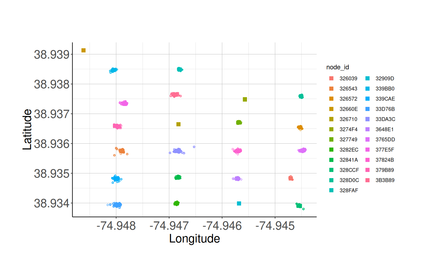
# Draw a map with the node locations
node_map <- map_node_locations(node_locs, tile_url = my_tile_url)
node_map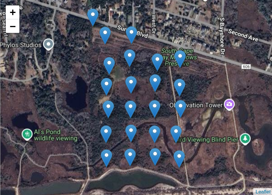
8.4 Load Station Detection Data
These are your tag detections in the ‘raw’ or ‘blu’ data tables in your database.
# Load from DB
con <- DBI::dbConnect(duckdb::duckdb(),
                      dbdir = database_file,
                      read_only = TRUE)

# load raw data table into RStudio and filter it based on start and stop time
detection_df <- tbl(con, "raw") |>
  filter(time >= det_start_time && time <= det_stop_time) |>
  filter(tag_id == selected_tag_id) |>
  collect()

# disconnect from the databse
DBI::dbDisconnect(con)

# create time_value variable
detection_df <- detection_df %>%
  mutate(time_value = as.integer(time))
8.5 Build a Grid
To actually quantify the amount of habitat an animal uses, we will create a 500x800 m grid and overlay it over the map. Each grid bin will be 5x5m.
# set the grid coordinates
grid_center_lat <- 38.93664800
grid_center_lon <- -74.9462
grid_size_x <- 500 # meters
grid_size_y <- 800 # meters
grid_bin_size <- 5 # meters

# Create a data frame with the details about the grid
grid_df <- build_grid(
  node_locs = node_locs,
  center_lat = grid_center_lat,
  center_lon = grid_center_lon,
  x_size_meters = grid_size_x,
  y_size_meters = grid_size_y,
  bin_size = grid_bin_size
)

# Draw all of the grid bins on a map
grid_map <- draw_grid(node_locs, grid_df)
grid_map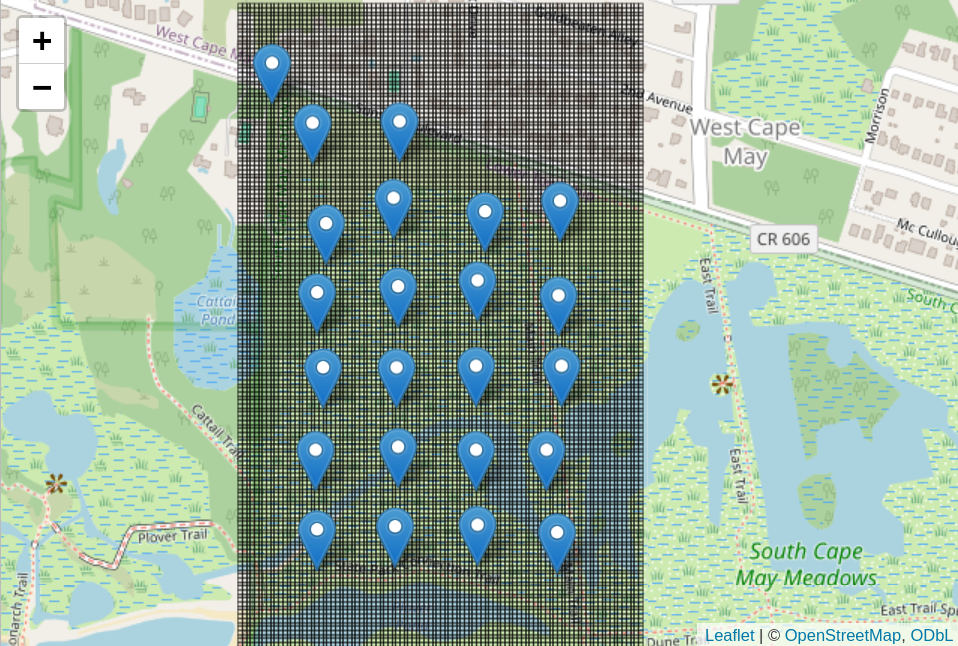
8.6 Calculate Locations
This will display the tag tracks and the tag location on the node grid map.
# create a locations dataframe with the calculate_track() function
locations_df <- calculate_track(
  start_time = "2023-10-04 23:00:00",
  # start_time = "2023-08-01 00:00:00",
  length_seconds = 6 * 3600,
  step_size_seconds = 15,
  det_time_window = 30, # Must have detection within this window to be included in position calculation
  filter_alpha = 0.7,
  filter_time_range = 60, # Time range to include detections in filtered value
  grid_df = grid_df,
  detection_df = detection_df,
  node_locs = node_locs,
  rssi_coefs = rssi_coefs,
  track_frame_output_path = NULL # If NULL no individual frames will be saved
)
print(locations_df)

# overlay the tag tracks on the node grid and satelitte picture
track_map <- map_track(node_locs,
                       locations_df,
                       my_tile_url)
track_map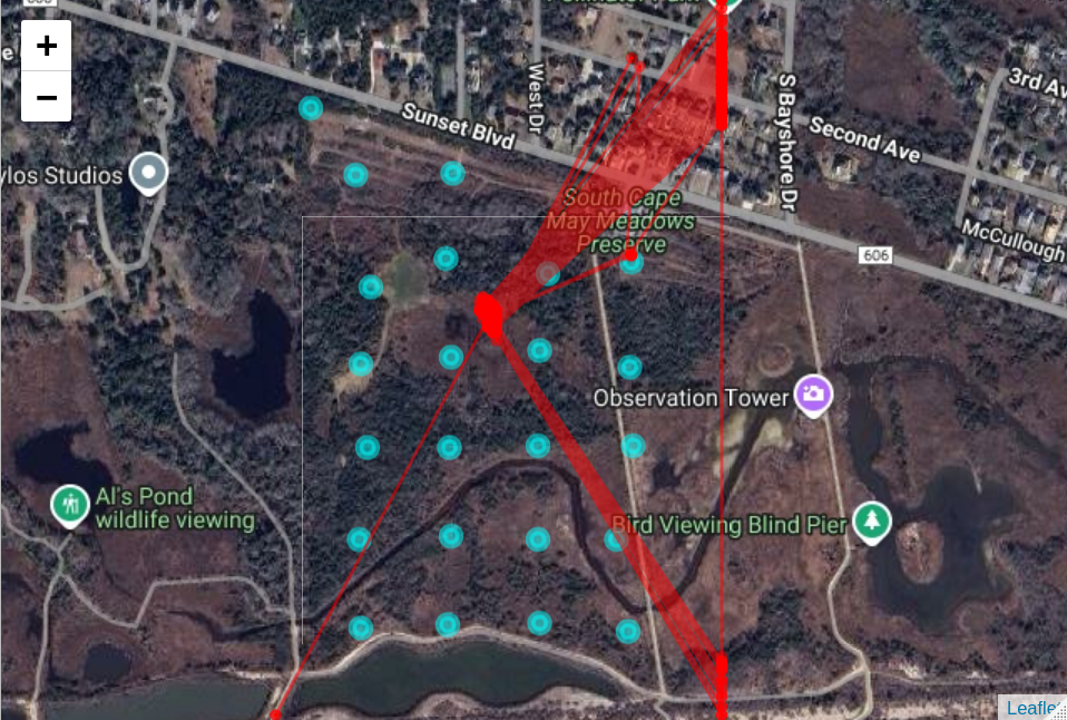
# calculate and display the location density on the node grid map
# source("R/functions/grid_search/grid_search_functions.R")
loc_density <- calc_location_density(grid_df = grid_df,
                                     locations_df = locations_df)

loc_density_map <- map_location_density(loc_density_df = loc_density, my_tile_url)
loc_density_map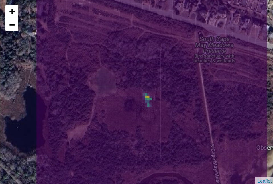
If you zoom in on the map, you can see the areas where the animal spent most of its time.
For tags with 1/8 wavelengths, you may need to use a lower RSSI coefficient to accurately map tracks and habitat use. Try using -115 for RSSI coefficient ‘a’.
Below is an example of a Power Tag with a 1/8 wave antenna, and will need a lower RSSI coefficient:
# Specify the RSSI vs Distance fit coefficients from calibration
a <- -115.0 # for 1/8 wave tags
b <- -59.03199894670
c <- 0.01188255653

rssi_coefs <- c(a, b, c)

# Selected Tag Id - Power Tag on a Swamp Sparrow (SWSP), 1/8 wave
selected_tag_id <- "2D4B782D"
Run the rest of the code blocks after setting these new RSSI coefficients to plot the habitat use of an individual with a 1/8 wave antenna.